QR code generator
In an attempt to learn something new, this time JavaScript, I have started coding small utility projects. First attempt at something which could be marginally useful, is a QR code generator. You can find it here bierlich.net/qr
There are many like it, but this one is mine.
Bibliographies from InspireHEP
The Inspire HEP tracks publications, conferences, job ads and many other things for high energy physics, and is in general an invaluable resource. One of its most useful features, is the fact that the API for their vast article database is open. With this in hand, it is easy to programmatically extract a bibliography for a high energy physics paper written in LaTeX, suitable for BibTeX.
I have written a small python script called citations.py, which does exactly that. I use it for all my papers, and put it here in the hope that other people will find it useful too.
You can download it as part of a physics paper template, which also includes some other functions -- handy when starting up a new paper, keeping you free of writing the boilerplate.
Clone it with
Call the script with:
will tell you all you need to know. Some key features are:
You need to use the inspireHEP citation keys when writing cite in your paper.
The script will scan through the .aux file produced by pdflatex for keys. This means that you can have several included .tex files, which will all be scanned (as opposed to the inspireHEP bibliography generator on their page, where you upload the tex files).
Should you need to add entries which are not tracked by inspire, you can make an auxiliary bibliography file, default name aux-bib.bib, but can be changed with an argument to the above call. Remember to add both to your manuscript.
Example use cases provided in the accompanying .tex files. Try to simply do make bib, and see what comes out.
Reverse tuning
In this post - which is really a jupyter notebook - I illustrate a cute principle of relevant for tuning of event generators. Under most circumstances, tuning refers to the process of fitting a large number of generator parameters to data. In that process, not all data should be weighted equally, and data points are assigned weights depending on how important their reproduction is deemed.
Consider now the reverse problem. We have a tune, which someone made at some point in the past, with weights unknown. Maybe they just guessed. It describes our data to some degree. We make a slight improvement of the model, and we now want to figure out if the "improvement" really makes things better, compared to the old one. It depends of course on our choice of weights. Since we don't know what weights were initially used, we have to try and re-estimate them. We therefore start out by fitting the weights, using the original tune as the target, and then make our comparison with the same weights.
In this constructed example we end up in a situation where this procedure renders our improvement worse than the original guess. Go figure.
import numpy as np
import matplotlib.pyplot as plt

np.random.seed(12)

# First generate some pseudo-data. This corresponds to real data from an experiment.
nd = 50 # Number of data points
x = np.linspace(0, 1, nd)
y = np.cos(x) + 0.3*np.random.rand(nd)
# Gaussian errors
errorsize = 0.15
yerr = abs(np.random.normal(0., errorsize, nd))

# Use a degree n polynomial with some given coefficients as our initial "tune"
degree = 4 # polynomial degree
coeffs = [-4.8, 8.6, -5.0, 0.8, 1.0]
#coeffs = [0.4, -1.4,  0.7, 1.0, 1.1]
# Our tune is then this
tune = np.poly1d(coeffs)

# And the "true" best fit in contrast.
w = [1 for i in range(0,nd)]
f = np.polyfit(x, y, degree, w=[ww * 1./np.sqrt(ye) for ww,ye in zip(w,yerr)])
p = np.poly1d(f)
print("Best fit (unit weights) coefficients = ")
print(f)

# Plot the stuff.
xplot = np.linspace(0, 1, 200)
plt.errorbar(x, y, yerr=yerr, fmt='o',color='black',label="Pseudo-data")
plt.plot(x,p(x),color='blue',label="Best fit (unit weights)")
plt.plot(x,tune(x),'--',color='red',label="Input tune")

plt.legend()
plt.show()

# We now want to figure out which weights we should use in the fit to reproduce "coeffs".
# That is: I want to get "coeffs" from the frame above as the result when I run np.polyfit.
import scipy.optimize as opt

# A chi2 function, taking the weights as an input
def chi2(weights):
    testCoeffs,cov = np.polyfit(x,y,degree,cov=True,w=[ww * 1./np.sqrt(ye) for ww,ye in zip(weights,yerr)])
    errs = np.diagonal(cov)
    chi2 = 0.
    for testC, targetC, err in zip(testCoeffs,coeffs, errs):
        chi2 += (targetC - testC)**2/err
    return chi2/float(degree)

# Here lies a challenge! If the initial guess on the weights
# is far away from the target, the fit will have a hard time converging.
# Maybe we can do better than standard minimization techniques. Genetic algorithm, maybe?
w0 = w
fittedWeights =  opt.minimize(chi2, w0, tol=1e-6)
# Let's take a look at the fitted weights
print("Fitted weights = ")
print(fittedWeights.x)

# And repeat the original fit with the new weights.
fOpt = np.polyfit(x, y, degree, w=[ww * 1./np.sqrt(ye) for ww,ye in zip(fittedWeights.x,yerr)])
pOpt = np.poly1d(fOpt)

print("Best fit (fitted weights) coefficients = ")
print(fOpt)
print("Best fit (unit weights) coefficients = ")
print(f)
print('The original "tune" = ')
print(coeffs)

# And plot the lot together
plt.errorbar(x, y, yerr=yerr, fmt='o',color='black',label="Pseudo-data")
plt.plot(x,pOpt(x),'-',color='green',label="Best fit (fitted weights)")
plt.plot(x,p(x),color='blue',label="Best fit (unit weights)")
plt.plot(x,tune(x),'--',color='red',label="Input tune")

plt.legend()
plt.show()

# Now we add a "better" model, and see if it improves the overall description of data.

# Get a global chi2 model vs. data, possibly weighted
def globalChi2(dataX, dataY, yerrs, model, weights=[]):
    if len(weights) ==0:
        weights = [1 for i in range(0,len(dataX))]
    mVals = [model(xx) for xx in dataX]
    chi2 = 0.
    sow = 0.
    for mv, target, te, w in zip(mVals, dataY, yerrs, weights):
        chi2 += w*(target - mv)**2/np.sqrt(te)
        sow+=w*np.sqrt(te)
    return chi2

w = [1 for i in range(0,nd)]
# First with unit weights
fImprovedUnit = np.polyfit(x, y, degree+1, w=[ww * 1./np.sqrt(ye) for ww,ye in zip(w,yerr)])
pImprovedUnit = np.poly1d(fImprovedUnit)
# Then with fitted weights
fImproved = np.polyfit(x, y, degree+1, w=[ww * 1./np.sqrt(ye) for ww,ye in zip(fittedWeights.x,yerr)])
pImproved = np.poly1d(fImproved)

print("Global GOF:")
print("Tune:")
print(globalChi2(x, y, yerr, tune))
print("Best fit unit weights:")
print(globalChi2(x, y, yerr, p))
print("Best fit fitted weights:")
print(globalChi2(x, y, yerr, pOpt))
print("Improved model unit weights:")
print(globalChi2(x, y, yerr, pImprovedUnit))
print("Improved model fitted weights:")
print(globalChi2(x, y, yerr, pImproved))

# And plot the lot together
plt.errorbar(x, y, yerr=yerr, fmt='o',color='black',label="Pseudo-data")
plt.plot(x,pOpt(x),'-',color='green',label="Best fit (fitted weights)")
plt.plot(x,p(x),color='blue',label="Best fit (unit weights)")
plt.plot(x,pImproved(x),'-',color='magenta',label="Improved model (fitted weights)")
plt.plot(x,pImprovedUnit(x),color='cyan',label="Improved model (unit weights)")
plt.plot(x,tune(x),'--',color='red',label="Input tune")

plt.legend()
plt.show()

Rivet tutorial for Electron-Ion collider
I did a tutorial on the Rivet analysis framework, mostly meant for people doing electron-proton collisions and electron-Ion collisions, but it can very well be used by anyone who wants a general introduction to the framework.
You can find a lecture note here, the associated slides here, as well as a video recording of the lecture on the tutorial page here.
Rivet for heavy ions
There is a new talk on the talks page. It is about a project which I have spent a large part of the past two years working on, called Rivet for heavy ions.
The project is based on the Rivet project, which is an analysis toolkit for high energy Monte Carlo simulations. The idea is that experimental papers are implemented in code, and one can then with the press of a button compare any Monte Carlo simulation to the results obtained in the paper. This is pretty valuable stuff, especially as Rivet has more than 400 analyses implemented.
What we have done in this project, is to extend the analysis toolkit to also handle heavy ion collisions. Time will tell if the toolkit will be as well received in the heavy ion community as in the pp community, but already now the initial investment is paying off in form of easy validation of our models.
The Glauber model
One of the staples of modeling of heavy ion collisions, is the Glauber model. It is one of the things all students have to go through starting out. The most remarkable thing about the Glauber model is its simplicity. It imposes a view of a proton-ion or ion-ion collisions, as the separate sub-collisions of several black disks. Some of the disks will interact, and some will not. This allows for a very inituitive understanding of a complicated system, as depicted below.
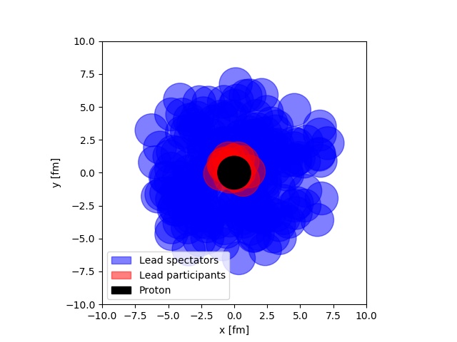
In the figure, a simulation of a proton-lead collision at LHC is depicted. The picture is taken from real simulation, that anyone with some introduction to Python programming can do. One of the other neat features of this model, is that it lends itself easily to computer implementation. If you are interesting in learning about this, I have written a small tutorial. that takes you through the most important steps of simulating the Glauber model, and using that simulation for an analysis.
To do the tutorial, simply download the pdf above and follow the steps, or you can pull the tutorial code directly using git, by doing:
git clone http://bierlich.net/git/glauber-tutorial.git
If you find any errors or misprints in the tutorial, I will appreciate it if you drop me a line.
PhD thesis
The PhD thesis. The crown on years of hard work. Also a document you seldom look at again after it is out. Should you, however, want to take a look in my thesis entitles Rope Hadronization, Geometry and Particle Production in pp and pA collisions, you can download it from the Lund University research portal.
Electrodynamics
The book Classical Electrodynamics by John David Jackson (3rd ed. Wiley) is one of the few true classics of theoretical physics, no matter what field you specialize in. And the problems in the book are interesting, but often quite difficult.
There are many people posting solutions to subsets of this book online - I only think mine are better, because I believe them to be correct. I hope they can prove useful to someone else, that's why I have compiled them into a solutions compendium.
Statistical physics
Statistical physics is fun, although I rarely get to use what I learned as a student. Once I calculated a bunch of the typical exercises, and took the time to write them up nicely. It is pretty standard stuff, entropy of a rubber band, van der Waals equation, and some more advanced stuff like RG equations, simple lattice spin model etc. It can be downloaded here.